XArray Example

To run this example, an environment.yml similar to this one could be used:

name: bh_xhistogram
channels:
  - conda-forge
dependencies:
  - python==3.8
  - boost-histogram
  - xhistogram
  - matplotlib
  - netcdf4

import xarray as xr
import numpy as np
import matplotlib.pyplot as plt
import numpy as np
import boost_histogram as bh
from xhistogram.xarray import histogram as xhistogram

Let’s look at using boost-histogram to imitate the xhistogram package by reading and producing xarrays. As a reminder, xarray is a sort of generalized Pandas library, supporting ND labeled and indexed data.

Simple 1D example

We will start with the first example from the xhistogram docs:

da = xr.DataArray(np.random.randn(100, 30), dims=["time", "x"], name="foo")
bins = np.linspace(-4, 4, 20)

xhistogram

And, this is what historamming and plotting looks like:

h = xhistogram(da, bins=[bins])
display(h)
h.plot()
# h is an xarray

<xarray.DataArray 'histogram_foo' (foo_bin: 19)>
array([  2,   1,   2,  22,  56, 135, 234, 375, 453, 496, 456, 346, 226,
        96,  65,  25,   7,   3,   0])
Coordinates:
  * foo_bin  (foo_bin) float64 -3.789 -3.368 -2.947 -2.526 ... 2.947 3.368 3.789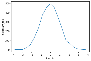

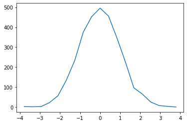
boost-histogram (direct usage)

Let’s first just try this by hand, to see how it works. This will not return an xarray, etc.

bh_bins = bh.axis.Regular(19, -4, 4)
bh_hist = bh.Histogram(bh_bins).fill(np.asarray(da).flatten())
plt.plot(bh_hist.axes[0].centers, bh_hist.values());

boost-histogram (adapter function)

Now, let’s make an adaptor for boost-histogram.

def bh_xhistogram(*args, bins):
    # Convert bins to boost-histogram axes first
    prepare_bins = (bh.axis.Variable(b) for b in bins)
    h = bh.Histogram(*prepare_bins)

    # We need flat NP arrays for filling
    prepare_fill = (np.asarray(a).flatten() for a in args)
    h.fill(*prepare_fill)

    # Now compute the xarray output.
    return xr.DataArray(
        h.values(),
        name="_".join(a.name for a in args) + "_histogram",
        coords=[
            (f"{a.name}_bin", arr.flatten(), a.attrs)
            for a, arr in zip(args, h.axes.centers)
        ],
    )

h = bh_xhistogram(da, bins=[bins])
display(h)
h.plot();

<xarray.DataArray 'foo_histogram' (foo_bin: 19)>
array([  2.,   1.,   2.,  22.,  56., 135., 234., 375., 453., 496., 456.,
       346., 226.,  96.,  65.,  25.,   7.,   3.,   0.])
Coordinates:
  * foo_bin  (foo_bin) float64 -3.789 -3.368 -2.947 -2.526 ... 2.947 3.368 3.789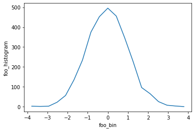

More features

Let’s add a few more features to our function defined above. * Let’s allow bins to be a list of axes or even a completely prepared histogram; this will allow us to take advantage of boost-histogram features later. * Let’s add a weights keyword so we can do weighted histograms as well.

def bh_xhistogram(*args, bins, weights=None):
    """
    bins is either a histogram, a list of axes, or a list of bins
    """

    if isinstance(bins, bh.Histogram):
        h = bins
    else:
        prepare_bins = (
            b if isinstance(b, bh.axis.Axis) else bh.axis.Variable(b) for b in bins
        )
        h = bh.Histogram(*prepare_bins)

    prepare_fill = (np.asarray(a).flatten() for a in args)

    if weights is None:
        h.fill(*prepare_fill)
    else:
        prepared_weights, *_ = xr.broadcast(weights, *args)
        h.fill(*prepare_fill, weight=np.asarray(prepared_weights).flatten())

    return xr.DataArray(
        h.values(),
        name="_".join(a.name for a in args) + "_histogram",
        coords=[
            (f"{a.name}_bin", arr.flatten(), a.attrs)
            for a, arr in zip(args, h.axes.centers)
        ],
    )

2D example

This also comes from the xhistogram docs.

# Read WOA using opendap
Temp_url = (
    "http://apdrc.soest.hawaii.edu:80/dods/public_data/WOA/WOA13/5_deg/annual/temp"
)
Salt_url = (
    "http://apdrc.soest.hawaii.edu:80/dods/public_data/WOA/WOA13/5_deg/annual/salt"
)
Oxy_url = (
    "http://apdrc.soest.hawaii.edu:80/dods/public_data/WOA/WOA13/5_deg/annual/doxy"
)

ds = xr.merge(
    [
        xr.open_dataset(Temp_url).tmn.load(),
        xr.open_dataset(Salt_url).smn.load(),
        xr.open_dataset(Oxy_url).omn.load(),
    ]
)

sbins = np.arange(31, 38, 0.025)
tbins = np.arange(-2, 32, 0.1)

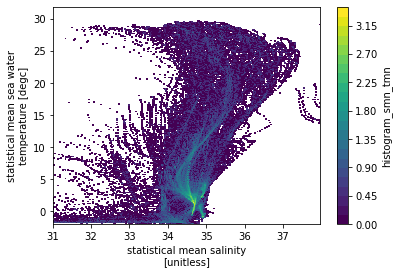
xhistogram

hTS = xhistogram(ds.smn, ds.tmn, bins=[sbins, tbins])
np.log10(hTS.T).plot(levels=31)

/usr/local/Caskroom/miniconda/base/envs/xtest/lib/python3.8/site-packages/xarray/core/computation.py:601: RuntimeWarning: divide by zero encountered in log10
  result_data = func(*input_data)

<matplotlib.collections.QuadMesh at 0x7f84c920b130>

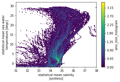
boost-histogram

We could hand in the same bin definitions, but let’s use boost-histogram axes instead:

sax = bh.axis.Regular(250, 31, 38)
tax = bh.axis.Regular(340, -2, 32)

hTS = bh_xhistogram(ds.smn, ds.tmn, bins=[sax, tax])
np.log10(hTS.T).plot(levels=31)

<matplotlib.collections.QuadMesh at 0x7f8528c132b0>

Speed comparson

%%timeit
hTS = xhistogram(ds.smn, ds.tmn, bins=[sbins, tbins])

17.6 ms ± 508 µs per loop (mean ± std. dev. of 7 runs, 100 loops each)

%%timeit
hTS = bh_xhistogram(ds.smn, ds.tmn, bins=[sax, tax])

4.7 ms ± 245 µs per loop (mean ± std. dev. of 7 runs, 100 loops each)

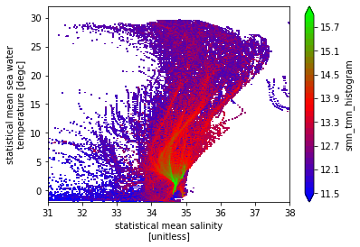
Weighted histogram

Let’s try a more complex example from the docs; the dVol weights one:

dz = np.diff(ds.lev)
dz = np.insert(dz, 0, dz[0])
dz = xr.DataArray(dz, coords={"lev": ds.lev}, dims="lev")

dVol = dz * (5 * 110e3) * (5 * 110e3 * np.cos(ds.lat * np.pi / 180))

hTSw = bh_xhistogram(ds.smn, ds.tmn, bins=[sax, tax], weights=dVol)
np.log10(hTSw.T).plot(levels=31, vmin=11.5, vmax=16, cmap="brg")

<matplotlib.collections.QuadMesh at 0x7f84b821c940>