Quickstart#

All of the examples will assume the following import:

import boost_histogram as bh

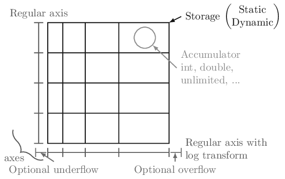
In boost-histogram, a histogram is collection of Axis objects and a storage.

Making a histogram#

You can make a histogram like this:

hist = bh.Histogram(bh.axis.Regular(bins=10, start=0, stop=1))

If you’d like to type less, you can leave out the keywords:

hist = bh.Histogram(bh.axis.Regular(10, 0, 1))

The exact same syntax is used for 1D, 2D, and ND histograms:

hist3D = bh.Histogram(
    bh.axis.Regular(10, 0, 100, circular=True),
    bh.axis.Regular(10, 0.0, 10.0),
    bh.axis.Variable([1, 2, 3, 4, 5, 5.5, 6]),
)

See Axes and Using Transforms.

You can also select a different storage with the storage= keyword argument; see Storages for details about the other storages.

Filling a histogram#

Once you have a histogram, you can fill it using .fill. Ideally, you should give arrays, but single values work as well:

hist = bh.Histogram(bh.axis.Regular(10, 0.0, 1.0))
hist.fill(0.9)
hist.fill([0.9, 0.3, 0.4])

Slicing and rebinning#

You can slice into a histogram using bin coordinates or data coordinates using bh.loc(v). You can also rebin with bh.rebin(n) or remove an entire axis using sum (technically as the third slice argument, though it is allowed by itself as well):

hist = bh.Histogram(
    bh.axis.Regular(10, 0, 1),
    bh.axis.Regular(10, 0, 1),
    bh.axis.Regular(10, 0, 1),
)
mini = hist[1:5, bh.loc(0.2) : bh.loc(0.9), sum]
# Will be 4 bins x 7 bins

See Indexing.

Accessing the contents#

You can use hist.values() to get a NumPy array from any histogram. You can get the variances with hist.variances(), though if you fill an unweighted storage with weights, this will return None, as you no longer can compute the variances correctly (please use a weighted storage if you need to). You can also get the number of entries in a bin with .counts(); this will return counts even if your storage is a mean storage. See Plotting.

If you want access to the full underlying storage, .view() will return a NumPy array for simple storages or a RecArray-like wrapper for non-simple storages. Most methods offer an optional keyword argument that you can pass, flow=True, to enable the under and overflow bins (disabled by default).

np_array = hist.view()

Setting the contents#

You can set the contents directly as you would a NumPy array; you can set either values or arrays at a time:

hist[2] = 3.5
hist[bh.underflow] = 0  # set the underflow bin
hist2d[3:5, 2:4] = np.eye(2)  # set with array

For non-simple storages, you can add an extra dimension that matches the constructor arguments of that accumulator. For example, if you want to fill a Weight histogram with three values, you can dimension:

hist[0:3] = [[1, 0.1], [2, 0.2], [3, 0.3]]

See Indexing.

Accessing Axes#

The axes are directly available in the histogram, and you can access a variety of properties, such as the edges or the centers. All properties and methods are also available directly on the axes tuple:

ax0 = hist.axes[0]
X, Y = hist.axes.centers

See Axes.

Saving Histograms#

You can save histograms using pickle:

import pickle

with open("file.pkl", "wb") as f:
    pickle.dump(h, f)

with open("file.pkl", "rb") as f:
    h2 = pickle.load(f)

assert h == h2

Special care was taken to ensure that this is fast and efficient. Please use the latest version of the Pickle protocol you feel comfortable using; you cannot use version 0, the version that was default on Python 2. The most recent versions provide performance benefits.

Computing with Histograms#

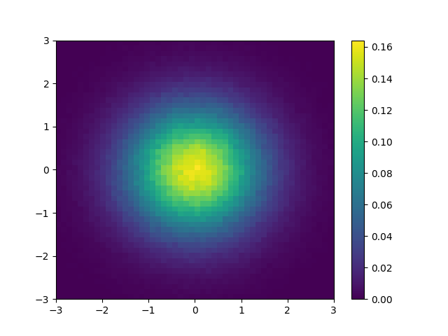
As an complete example, let’s say you wanted to compute and plot the density:

#!/usr/bin/env python3

from __future__ import annotations

import functools
import operator

import matplotlib.pyplot as plt
import numpy as np

import boost_histogram as bh

# Make a 2D histogram
hist = bh.Histogram(bh.axis.Regular(50, -3, 3), bh.axis.Regular(50, -3, 3))

# Fill with Gaussian random values
hist.fill(np.random.normal(size=1_000_000), np.random.normal(size=1_000_000))

# Compute the areas of each bin
areas = functools.reduce(operator.mul, hist.axes.widths)

# Compute the density
density = hist.view() / hist.sum() / areas

# Make the plot
fig, ax = plt.subplots()
mesh = ax.pcolormesh(*hist.axes.edges.T, density.T)
fig.colorbar(mesh)
plt.savefig("simple_density.png")

Comparing with Boost.Histogram#

This is built on the Boost.Histogram library.

See Comparison with Boost.Histogram.

Quickstart

Contents